

NumPy - Data Science
2. The Shape and Reshaping of NumPy Array
a. Dimensions of NumPy array
You can easily determine the number of dimensions or axes of a NumPy array using the ndims attribute:
# number of axis
a = np.array([[5,10,15],[20,25,20]])
print('Array :','\n',a)
print('Dimensions :','\n',a.ndim)
This array has two dimensions: 2 rows and 3 columns.
b. Shape of NumPy array
The shape is an attribute of the NumPy array that shows how many rows of elements are there along each dimension. You can further index the shape so returned by the ndarray to get value along each dimension:
a = np.array([[1,2,3],[4,5,6]])
print('Array :','\n',a)
print('Shape :','\n',a.shape)
print('Rows = ',a.shape[0])
print('Columns = ',a.shape[1])
c. Size of NumPy array
You can determine how many values there are in the array using the size attribute. It just multiplies the number of rows by the number of columns in the ndarray:
# size of array
a = np.array([[5,10,15],[20,25,20]])
print('Size of array :',a.size)
print('Manual determination of size of array :',a.shape[0]*a.shape[1])

d. Reshaping a NumPy array
Reshaping a ndarray can be done using the np.reshape() method. It changes the shape of the ndarray without changing the data within the ndarray:
# reshape
a = np.array([3,6,9,12])
np.reshape(a,(2,2))
Here, I reshaped the ndarray from a 1-D to a 2-D ndarray.
While reshaping, if you are unsure about the shape of any of the axis, just input -1. NumPy automatically calculates the shape when it sees a -1:
a = np.array([3,6,9,12,18,24])
print('Three rows :','\n',np.reshape(a,(3,-1)))
print('Three columns :','\n',np.reshape(a,(-1,3)))
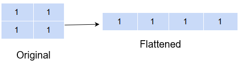
e. Flattening a NumPy array
Sometimes when you have a multidimensional array and want to collapse it to a single-dimensional array, you can either use the flatten() method or the ravel() method:
a = np.ones((2,2))
b = a.flatten()
c = a.ravel()
print('Original shape :', a.shape)
print('Array :','\n', a)
print('Shape after flatten :',b.shape)
print('Array :','\n', b)
print('Shape after ravel :',c.shape)
print('Array :','\n', c)
Original shape : (2, 2) Array : [[1. 1.] [1. 1.]] Shape after flatten : (4,) Array : [1. 1. 1. 1.] Shape after ravel : (4,) Array : [1. 1. 1. 1.]
But an important difference between flatten() and ravel() is that the former returns a copy of the original array while the latter returns a reference to the original array. This means any changes made to the array returned from ravel() will also be reflected in the original array while this will not be the case with flatten().
b[0] = 0
print(a)
[[1. 1.]
 [1. 1.]]
The change made was not reflected in the original array.
c[0] = 0
print(a)
[[0. 1.] [1. 1.]]
But here, the changed value is also reflected in the original ndarray.
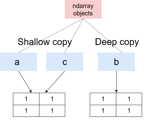
What is happening here is that flatten() creates a Deep copy of the ndarray while ravel() creates a Shallow copy of the ndarray.
Deep copy means that a completely new ndarray is created in memory and the ndarray object returned by flatten() is now pointing to this memory location. Therefore, any changes made here will not be reflected in the original ndarray.
A Shallow copy, on the other hand, returns a reference to the original memory location. Meaning the object returned by ravel() is pointing to the same memory location as the original ndarray object. So, definitely, any changes made to this ndarray will also be reflected in the original ndarray too.
f. Transpose of a NumPy array
Another very interesting reshaping method of NumPy is the transpose() method. It takes the input array and swaps the rows with the column values, and the column values with the values of the rows:
a = np.array([[1,2,3],
[4,5,6]])
b = np.transpose(a)
print('Original','\n','Shape',a.shape,'\n',a)
print('Expand along columns:','\n','Shape',b.shape,'\n',b)On transposing a 2 x 3 array, we got a 3 x 2 array. Transpose has a lot of significance in linear algebra.

0 Comments